python --version
   

   python3 --version
   

conda create --name hw4 python=3.12

conda activate hw4

Markov decision processes (MDPs) can be used to model situations with uncertainty (which is most of the time in the real world). In this assignment, you will implement algorithms to find the optimal policy, both when you know the transitions and rewards (value iteration) and when you don't (reinforcement learning). You will use these algorithms on Mountain Car, a classic control environment where the goal is to control a car to go up a mountain.

Problem 1: Value Iteration

In this problem, you will perform value iteration updates manually on a basic game to build your intuitions about solving MDPs. The set of possible states in this game is $\text{States} = \{-2, -1, 0, +1, +2\}$ and the set of possible actions is $\text{Actions}(s) = \{a_1, a_2\}$ for all states that are not end states. The starting state is $0$ and there are two end states, $-2$ and $+2$. Recall that the transition function $T: \text{States} \times \text{Actions} \rightarrow \Delta(\text{States})$ encodes the probability of transitioning to a next state $s'$ after being in state $s$ and taking action $a$ as $T(s'|s,a)$. In this MDP, the transition dynamics are given as follows:

$\forall i \in \{-1, 0, 1\} \subseteq \text{States}$,

• $T(i-1 | i, a_1) = 0.8$ and $T(i+1 | i, a_1) = 0.2$
• $T(i-1 | i, a_2) = 0.7$ and $T(i+1 | i, a_2) = 0.3$

1. What is the value of $V^\star_i(s)$ for each $s \in \text{States}$ after each iteration $i = \{1, 2\}$ of value iteration? Recall that $\forall s \in \text{States}$, $V^\star_0(s) = 0$ and, for any $i$, end state $s_{\text{end}}$, we have $V^\star_i(s_\text{end}) = 0$.
   The $V^\star_i(s)$ of all 5 states after each iteration. In total, 10 values should be reported.
2. Using $V^\star_2(\cdot)$, what is the corresponding optimal policy $\pi^\star$ for all non-end states?
   Optimal policy $\pi^\star(s)$ for each non-end state.

Problem 2: Transforming MDPs

In computer science, the idea of a reduction is very powerful: say you can solve problems of type A, and you want to solve problems of type B. If you can convert (reduce) any problem of type B to type A, then you automatically have a way of solving problems of type B potentially without doing much work! We saw an example of this for search problems when we reduce A* to UCS. Now let's do it for solving MDPs.

1. Suppose we have an MDP with states $\text{States}$ and a discount factor $\gamma < 1$, but we have an MDP solver that can only solve MDPs with discount factor of $1$. How can we leverage this restricted MDP solver to solve the original MDP?

   Let us define a new MDP with states $\text{States}' = \text{States} \cup \{ o \}$, where $o$ is a new state. Let's use the same actions ($\text{Actions}'(s) = \text{Actions}(s)$), but we need to keep the discount $\gamma' = 1$. Your job is to define transition probabilities $T'(s' | s, a)$ and rewards $\text{Reward}'(s, a, s')$ for the new MDP in terms of the original MDP such that the optimal values $V_\text{opt}(s)$ for all $s \in \text{States}$ are equal under the original MDP and the new MDP.

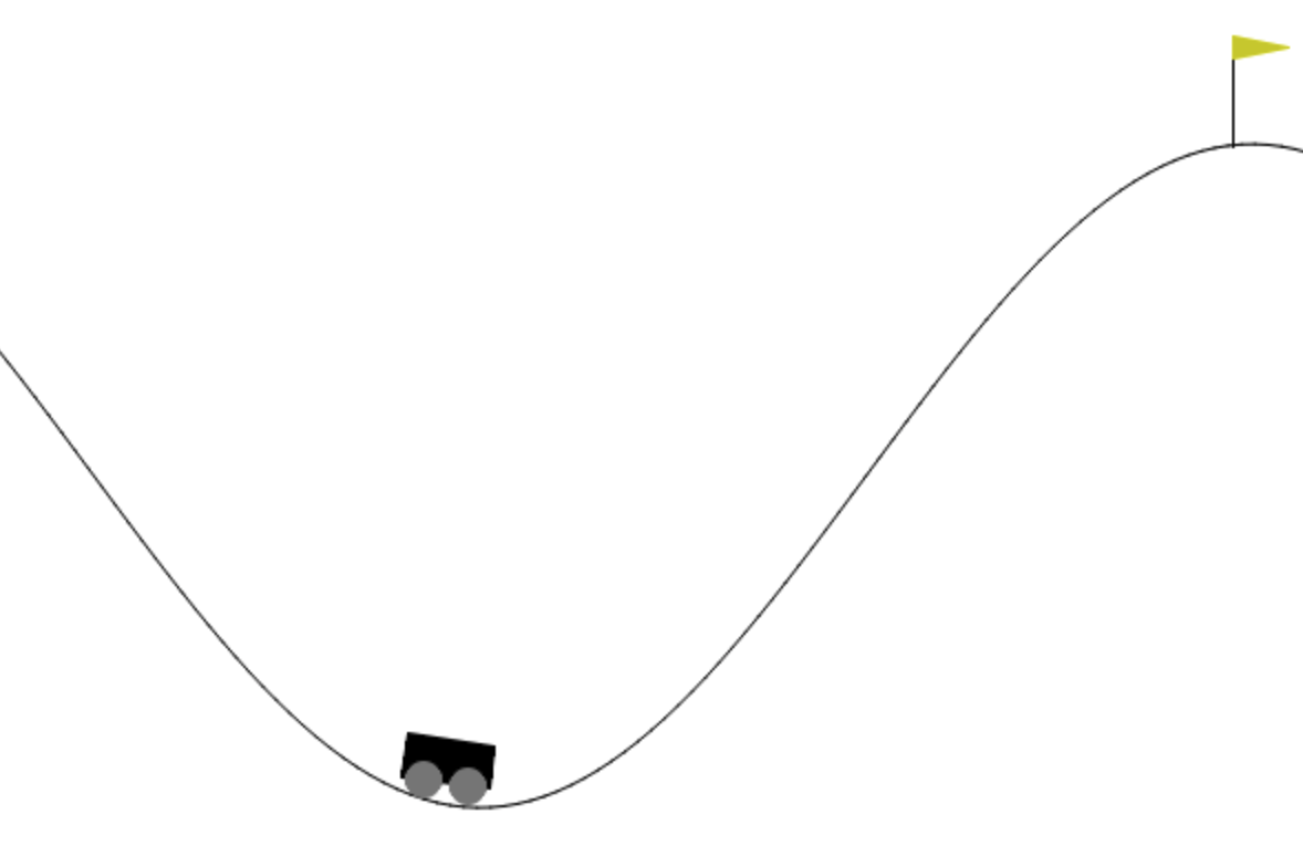
   Hint: If you're not sure how to approach this problem, go back to the slide notes from this MDP lecture and closely read the slides on convergence toward the end of the deck.
   Transition probabilities ($T'$) and reward function ($\text{Reward}'$) written in mathematical expressions, followed by a short proof to show that the two optimal values are equal. Use consistent notation from the question.

Problem 3: Value Iteration on Mountain Car

Now that we have gotten a bit of practice with general-purpose MDP algorithms, let's use them for some control problems. Mountain Car is a classic example in robot control [7] where you try to get a car to the goal located on the top of a steep hill by accelerating left or right. We will use the implementation provided by The Farama Foundation's Gymnasium, formerly OpenAI Gym.

The state of the environment is provided as a pair (position, velocity). The starting position is randomized within a small range at the bottom of the hill. At each step, the actions are either to accelerate to the left, to the right, or do nothing, and the transitions are determined directly from the physics of a frictionless car on a hill. Every step produces a small negative reward, and reaching the goal provides a large positive reward.

First, install all the dependencies needed to get Mountain Car running in your environment. Note that we are using Python 3.12 for this assignment. If you are getting "module not found" errors after downloading all the requirements, try using `pip` instead of `pip3` and `python` instead of `python3`.

pip3 install -r requirements.txt

Then to get the feel for the environment, test with an untrained agent which takes random action at each step and see how it performs.

python3 mountaincar.py --agent naive

You will see the agent struggling, not able to complete the task within the time limit. In this assignment, you will train this agent with different reinforcement learning algorithms so that it can learn to climb the hill. As the first step, we have designed two MDPs for this task. The first uses the car's continuous (position, velocity) state as is, and the second discretizes the position and velocity into bins and uses indicator vectors. Carefully examine ContinuousGymMDP and DiscreteGymMDP classes in util.py and make sure you understand.

If we want to apply value iteration to the DiscreteGymMDP (think about why we can't apply it to ContinuousGymMDP), we require the transition probabilities $T(s, a, s')$ and rewards $R(s, a, s')$ to be known. But oftentimes in the real world, $T$ and $R$ are unknown, and the gym environments are set up in this way as well, only interfacing through the .step() function. One method to still determine the optimal policy is model-based value iteration, which runs Monte Carlo simulations to estimate $\hat{T}$ and $\hat{R}$, and then runs value iteration. This is an example of model-based RL. Examine RLAlgorithm in util.py to understand the getAction and incorporateFeedback interface and peek into the simulate function to see how they are called repeatedly when training over episodes.

1. As a warm up, we will start with implementing value iteration as you learned in lectures, and run it on the number line MDP from Problem 1. Complete valueIteration function in submission.py.
2. Now in submission.py, implement ModelBasedMonteCarlo which runs valueIteration every calcValIterEvery steps that the RL agent operates. The getAction method controls how we use the latest policy as determined by value iteration, and the incorporateFeedback method updates the transition and reward estimates, calling value iteration when needed. Implement the getAction and incorporateFeedback methods for ModelBasedMonteCarlo.
3. Run python3 train.py --agent value-iteration to train the agent using model based value iteration you implemented above and see the plot of reward per episode. Comment on the plot, and discuss when might model based value iteration perform poorly. If your plot is not converging, double check your implementation of incorporateFeedback. You can also run python3 mountaincar.py --agent value-iteration to visually observe how the trained agent performs the task now.
   
   Note: RL algorithms, whether model-based or model-free, are generally unstable in high-dimensional environments. Correct algorithms do not always converge, depending on subtle differences in implementation and random seeds. The teaching staff has tested on various correct implementations and found that $\texttt{random.seed(2)}$ or $\texttt{random.seed(5)}$ in L74 of $\texttt{train.py}$ worked for these implementations. If you don't see the reward improving after 200-300 iterations, feel free to change this line.
   Plot of reward and 2-3 sentences describing the plot and discussion of when model based value iteration may fail.

Problem 4: Q-Learning Mountain Car

In the previous question, we've seen how value iteration can take an MDP which describes the full dynamics of the game and return an optimal policy, and we've also seen how model-based value iteration with Monte Carlo simulation can estimate MDP dynamics if unknown at first and then learn the respective optimal policy. But suppose you are trying to control a complex system in the real world where trying to explicitly model all possible transitions and rewards is intractable. We will see how model-free reinforcement learning can nevertheless find the optimal policy.

1. For a discretized MDP, we have a finite set of (state, action) pairs. We learn the Q-value for each of these pairs using the Q-learning update learned in class. In the TabularQLearning class, implement the getAction method which selects action based on explorationProb, and the incorporateFeedback method which updates the Q-value given a (state, action) pair.
2. For Q-learning in continuous states, we need to use function approximation. The first step of function approximation is extracting features given state. Feature extractors of different complexities work well with different problems: linear and polynomial feature extractors that work well with simpler problems may not be suitable for other problems. For the mountain car task, we are going to use a Fourier feature extractor. As background, any continuous periodic function can be approximated as a Fourier Series $$f(x) = \frac{a_0}{2} + \sum_{j=1}^n\left[a_j\cos(2\pi j x/T) + b_j\sin(2\pi j x/ T)\right]$$ with $a_j$ and $b_j$ sequences of coefficients determined by integrating $f$. To apply this to Q-learning with function approximation, we want the learned weights $w$ to emulate $a_j$ and $b_j$ and the output of $\phi$ to provide the basis of varying sinusoid periods as seen in $\cos(2\pi j x/T)$ for $j = 1, 2, \ldots, n$ [1]. Thus, for state $s = [s_1, s_2, \ldots, s_k]$ and maximum coefficient $m$, the feature extractor $\phi$ is: $$\phi(s, m) = [\cos(0), \cos(\pi s_1), \ldots, \cos(\pi s_k), \cos(2\pi s_1), \cos(\pi(s_1+s_2)), \ldots, \cos(\pi(ms_1 + ms_2 + \ldots + ms_k))]$$ $$= \left\{\cos\left(\sum_{i=1}^k c_i \pi s_i\right): \forall c_1\in\mathscr{C}, \ldots, c_k\in\mathscr{C}\right\}$$ where $\mathscr{C} = \{0, 1, \ldots, m\}$ is the set of non-negative integers from 0 to $m$. Note that $\phi(s, m) \in \mathbb{R}^{(m+1)^k}$. For those interested, look up Fourier approximation and how effective Fourier features are in different settings.
   
   Note that in the code you implement, there is another variable $\texttt{scale}$ which is applied to different dimensions of the input state. We give you an example of how to compute this Fourier feature with $s = (x, y)$, $\texttt{scale} = [d_1, d_2]$ and $m = 2$. We find all the entries by considering all the combinations of scaled entries of the state as below.

   	0	$$d_1x$$	$$2d_1x$$
   0	0	$d_1x$	$2d_1x$
   $d_2y$	$d_2y$	$d_1x + d_2y$	$2d_1x + d_2y$
   $2d_2y$	$2d_2y$	$d_1x + 2d_2y$	$2d_1x + 2d_2y$

   
   Our feature extractor will return all these 9 elements, after multiplying by $\pi$ and applying cosine. For a higher dimensional state, we will repeat this "outer-sum" with the nine entries from the previous sum and three entries for the next dimension. Implement fourierFeatureExtractor in submission.py. Looking at util.polynomialFeatureExtractor may be useful for familiarizing oneself with numpy.
3. Now we can find the Q-value of each (state, action) by multiplying the extracted features from this pair with weights. Unlike the tabular Q-learning in which Q-values are updated directly, with function approximation, we are updating weights associated with each feature. Using fourierFeatureExtractor from the previous part, complete the implementation of FunctionApproxQLearning.
4. Run python3 train.py --agent tabular and python3 train.py --agent function-approximation to see the plots for how the TabularQLearning and FunctionApproxQLearning work respectively, and comment on the plots. If your plot is not converging, double check your implementation of incorporateFeedback. You should expect to see that tabular Q-learning performs better than function approximation Q-learning on this task. What might be some of the reasons? You can also run python3 mountaincar.py --agent tabular and python3 mountaincar.py --agent function-approximation to visualize the agent trained with continuous and discrete MDP respectively.
Plots and 2-3 sentences comparing the performances of TabularQLearning and FunctionApproxQLearning, discussing possible reasons as well.
5. What are some possible benefits of function approximation Q-learning for mountain car or other environments? Consider the situations where the exploration period is limited, where the state space is very high dimensional and difficult to explore, and/or you have space constraints.
2-3 sentences discussing why FunctionApproxQLearning can be better in various scenarios.

Problem 5: Safe Exploration

We learned about different state exploration policies for RL in order to get information about $(s, a)$. The method implemented in our MDP code is epsilon-greedy exploration, which balances both exploitation (choosing the action $a$ that maximizes $\hat{Q}_{\text{opt}}(s, a))$ and exploration (choosing the action $a$ randomly). $$\pi_{\text{act}}(s) = \begin{cases} \arg\max_{a \in \text{Actions}}\hat{Q}_{\text{opt}}(s,a) & \text{probability } 1 - \epsilon \\ \text{random from Actions}(s) & \text{probability } \epsilon \end{cases}$$

In real-life scenarios when safety is a concern, there might be constraints that need to be set in the state exploration phase. For example, robotic systems that interact with humans should not cause harm to humans during state exploration. Safe exploration in RL is thus a critical research question in the field of AI safety and human-AI interaction [2]. You can learn more about safe exploration in this week's ethics contents.

Safe exploration can be achieved via constrained RL. Constrained RL is a subfield of RL that focuses on optimizing agents' policies while adhering to predefined constraints - in order to ensure that certain unsafe behaviors are avoided during training and execution.

Assume there are harmful consequences for the driver of the Mountain Car if the car exceeds a certain velocity. One very simple approach of constrained RL is to restrict the set of potential actions that the agent can take at each step. We want to apply this approach to restrict the states that the agent can explore in order to prevent reaching unsafe speeds.

1. The implementation of the Mountain Car MDP you built in the previous questions actually already has velocity constraints in the form of a self.max_speed parameter. Read through OpenAI Gym's Mountain Car implementation and explain how self.max_speed is used.
   One sentence on how self.max_speed parameter is used in mountain_car.py
2. Run Function Approximation Q-Learning without the max_speed constraint by running python3 train.py --agent function-approximation --max_speed=100000. We are changing max_speed from its original value of 0.07 to a very large float to approximate removing the constraint entirely. Notice that running the MDP unconstrained doesn't really change the output behavior. Explain in 1-2 sentences why this might be the case.
   One sentence explaining why the Q-Learning result doesn't necessarily change.
3. Consider a different way of setting the constraint where you limit the set of actions the agent can take in the action space. In ConstrainedQLearning, implement constraints on the set of actions the agent can take each step such that velocity_(t+1) < velocity_threshold. Remember to handle the case where the set of valid actions is empty. Below is the equation that Mountain Car uses to calculate velocity at time step $t+1$ (the equation is also provided here). $$\text{velocity}_{t+1} = \text{velocity}_t + (\text{action} - 1) * \text{force} - \cos(3 * \text{position}_t) * \text{gravity}$$ We've determined that in the mountain car environment, a velocity of 0.065 is considered unsafe. After implementing the velocity constraint, run grader test 5c-helper to examine the optimal policy for two continuous MDPs running Q-Learning (one with max_speed of 0.065 and the other with a very large max_speed constraint). Provide 1-2 sentences explaining why the output policies are now different.
   Complete the implementation of ConstrainedQLearning in submission.py, then run python3 grader.py 5c-helper. Include 1-2 sentences explaining the difference in the two scenarios.
4. The concept of safe exploration in RL extends to other real-world contexts where some amount of learning through trial and error might be expected. One example of this is clinical research: conducting epsilon-greedy exploration examining the effects of a drug that has serious or fatal side effects may harm a lot of people and be ethically questionable. For example, one of the most notorious cases of abuse in clinical trials was the Tuskegee Syphilis Study conducted between 1932 and 1972 by the US Public Health Service and the CDC [3]. During the study, 400 African American men with Syphilis were not treated so that researchers could study the progression of the disease, costing many of these individuals their lives. As a result, ethical guidelines have been put in place to guide research involving human-beings, like clinical research [4][5]. Many of these guidelines apply to other research contexts beyond medicine. In many ways, these guardrails for science are similar to the constraints you set for Mountain Car to keep its velocity within a safe range.

   The Belmont report, one of the list of guidelines for conducting human-subjects research that arose after the Tuskegee Syphilis Study, lists three principles: Respect for Persons, Beneficence, and Justice [3]. In 2012, the US Department of Homeland Security applied these principles to describe how to conduct ethical information and communication technology research in the Menlo Report [6]. The principles are as follows:

   • Respect for persons: Participation as a research subject is voluntary, and follows from informed consent; Treat individuals as autonomous agents and respect their right to determine their own best interests; Respect individuals who are not targets of research yet are impacted; Individuals with diminished autonomy, who are incapable of deciding for themselves, are entitled to protection.
   • Beneficence: Do not harm; Maximize probably benefits and minimize probable harms; Systematically assess both risk of harm and benefit.
   • Justice: Each person deserves equal consideration in how to be treated, and the benefits of research should be fairly distributed according to individual need, effort, societal consideration, and merit; Selection of subjects should be fair, and burdens should be allocated equitably across impacted subjects.
   • Respect for Law and Public Interest: Engage in legal due diligence; Be transparent in methods and results; Be accountable for actions.
   Imagine a company is working on testing and improving their autonomous driving technology through RL. They want to run their experiments on streets in residential neighborhoods. Describe an MDP (specifically define $\text{States}$, $\text{Actions}(s)$, and $\text{Reward}(s, a, s')$) and a state exploration policy that would potentially cause harm to humans. Which of the 4 Menlo Report principles might be violated by running this experiment and why? Explain in 1-3 sentences.
   Definition of an MDP's $\text{States}$, $\text{Actions}(s)$, and $\text{Reward}(s, a, s')$, a state exploration policy, and a relevant Menlo Report principle that might be violated with an explanation.

[1] Konidaris et al. Value Function Approximation in Reinforcement Learning using the Fourier Basis. AAAI. 2011.

[2] OpenAI. Benchmarking Safe Exploration in Deep Reinforcement Learning

[3] The Centers for Disease Control and Prevention. The Untreated Syphilis Study at Tuskegee Timeline.

[4] The US Department of Health and Human Services. The Belmont Report. 1978.

[5] The World Medical Association. The Declaration of Helsinki. 1964.

[6] The US Department of Homeland Security. The Menlo Report. 2012.

[7] Moore. Efficient Memory-based Learning for Robot Control. 1990.